

[ad_1]
One would possibly usually ponder the necessity to perceive and study Inventory Market Maths.
What’s the have to study Maths for inventory markets?The place do I study in regards to the software of maths within the inventory markets?What are the fundamentals of inventory market maths?That are the ideas to focus on whereas studying inventory market maths?
Many goal to study algorithmic buying and selling from a mathematical viewpoint. Varied mathematical ideas, statistics, and econometrics play an important function in giving your inventory buying and selling that edge within the inventory market.
Here is an entire record of all the things that we’re overlaying about Inventory Market maths on this weblog:
What’s inventory market maths?
Within the inventory market, the maths used contains the ideas and calculations used to analyse and perceive inventory market behaviour, assess funding alternatives, and handle threat. It features a vary of strategies and instruments that traders and merchants use to make knowledgeable choices.
Shifting forward, allow us to discover out extra about algorithmic buying and selling and its affiliation with Arithmetic.
An summary of algorithmic buying and selling
Algorithmic buying and selling makes use of laptop algorithms to automate and execute trades at excessive speeds. It depends on quantitative information to make knowledgeable choices, eradicating feelings from buying and selling. Methods embody development following, arbitrage, and market making. Whereas it provides pace and effectivity, it additionally includes dangers like technical failures and requires fixed monitoring. Efficient algo buying and selling calls for robust technical abilities, entry to real-time information, and adherence to market rules.
The video under supplies an summary of statistical arbitrage buying and selling at Quantra:
Additionally, here’s a temporary market making video which might be rapidly explored:
Subsequent, we’ll discover out what algorithmic buying and selling maths means.
What’s algorithmic buying and selling math?
Algorithmic buying and selling maths refers back to the mathematical fashions and strategies used within the design and implementation of algorithms that automate the buying and selling of monetary devices. This area combines ideas from arithmetic, statistics, laptop science, and finance to create methods that may execute trades at excessive speeds and frequencies with minimal human intervention. The first purpose is to handle dangers by exploiting market inefficiencies.
However why does algorithmic buying and selling require maths and what’s the relevance of the identical? Allow us to discover out the reply to this query subsequent.
Why does Algorithmic Buying and selling require math?
Algorithmic buying and selling requires math to successfully analyse and predict market actions. Methods like monetary time collection evaluation and regression assist in understanding historic information and forecasting future tendencies. Mathematical fashions present the inspiration for machine studying algorithms, which determine patterns and make predictions based mostly on historic information.
Danger administration is one other crucial space the place math is crucial. Quantifying threat includes utilizing fashions reminiscent of Worth at Danger (VaR) and performing stress checks to grasp potential losses. Optimisation strategies, usually grounded in mathematical theories like Fashionable Portfolio Idea (MPT), are used to allocate belongings in a method that balances threat and return.
Pricing and valuation of monetary devices, particularly derivatives, rely closely on mathematical fashions. Calculus and stochastic processes, as an illustration, are used within the Black-Scholes mannequin for choice pricing, which helps in figuring out the truthful worth of derivatives based mostly on their underlying belongings.
Execution algorithms, which decide the optimum approach to execute trades to minimise market impression and prices, additionally rely on math. Fashions like VWAP (Quantity Weighted Common Worth) and TWAP (Time Weighted Common Worth) use mathematical formulation to interrupt massive orders into smaller ones over time, making certain higher execution high quality.
Shifting forward, we’ll learn how arithmetic grew to become so vital within the buying and selling area.
When and How Arithmetic grew to become fashionable in buying and selling: A historic tour
In 1967, Edward Thorp, a arithmetic professor on the College of California, printed “Beat the Market”, claiming to have a foolproof methodology for inventory market success based mostly on his blackjack system. This technique concerned promoting shares and bonds at one value and repurchasing them at a lower cost, main Thorp to ascertain the profitable hedge fund Princeton/Newport Companions. The technique’s reputation drew physicists to finance, considerably impacting Wall Avenue.
Now allow us to head to the Mathematical ideas for algorithmic buying and selling that are the core of this text.
Mathematical Ideas for Inventory Markets
Beginning with the mathematical for inventory buying and selling, it’s a should to say that mathematical ideas play an vital function in algorithmic buying and selling. Allow us to check out the broad classes of various mathematical ideas right here:
Descriptive Statistics
Allow us to stroll by way of descriptive statistics, which summarize a given information set with temporary descriptive coefficients. These is usually a illustration of both the entire or a pattern from the inhabitants.

Measure of Central Tendency
Right here, Imply, Median and Mode are the essential measures of central tendency. These are fairly helpful in terms of taking out common worth from a knowledge set consisting of assorted values. Allow us to perceive every measure one after the other.
Imply
This one is essentially the most used idea within the numerous fields regarding arithmetic and in easy phrases, it’s the common of the given dataset. Thus, if we take 5 numbers in a knowledge set, say, 12, 13, 6, 7, 19, 21, the system of the imply is
$$frac{x_1 + x_2 +x_3 + …….x_n}{n}$$
which makes it:(12 + 13 + 6 + 7 + 19 + 21)/6 = 13
Moreover, the dealer tries to provoke the commerce on the premise of the imply (transferring common) or transferring common crossover.
Right here, allow us to perceive two kinds of transferring averages based mostly on the ranges (variety of days) of the time interval they’re calculated in and the transferring common crossover:
1. Quicker transferring common (Shorter time interval): A sooner transferring common is the imply of a knowledge set (inventory costs) calculated over a brief time period, say previous 20 days.
2. Slower transferring common (Longer time interval): A slower transferring common is the one that’s the imply of a knowledge set (inventory costs) calculated from an extended time interval say 50 days. Now, a faster-moving common and a slower transferring common additionally come to a place collectively the place a “crossover” happens.
“A crossover happens when a faster-moving common (i.e., a shorter interval transferring common) crosses a slower transferring common (i.e. an extended interval transferring common). In different phrases, that is when the shorter interval transferring common line crosses an extended interval transferring common line.” ⁽¹⁾
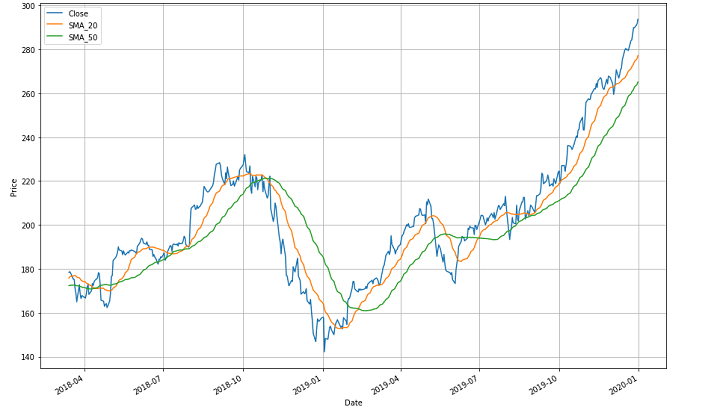
Right here to elucidate it higher, the graph picture above reveals three transferring strains. The blue one reveals the worth line over the talked about interval. The inexperienced one signifies a slower-moving common of fifty days and the orange one signifies a faster-moving common of 20 days between April 2018 and January 2020.
Now beginning with the inexperienced line, (slower transferring common) the complete development line reveals the various technique of inventory costs over longer time intervals. The development line follows a zig-zag sample and there are totally different crossovers.
For instance, there’s a crossover between October 2018 and January 2019 the place the orange line (faster-moving common) comes from above and crosses the inexperienced one (slower-moving common) whereas taking place. This means that any particular person or agency can be promoting the shares at this level because it reveals a stoop available in the market. This crossover level known as the “assembly level”.
After the assembly level, forward each the strains go down after which go up after some extent to create yet one more (after which one other) crossover(s). Since there are lots of crossovers within the graph, it is best to be capable to determine every of them by yourself now.
Now, it is extremely vital to notice right here that the “assembly level” is taken into account bullish if the faster-moving common crosses over the slower-moving common and goes past within the upward route.Quite the opposite, it’s thought-about bearish if the faster-moving common drops under the slower-moving common and goes past. That is so as a result of within the former situation, it reveals that in a short while, there got here an upward development for specific shares. Whereas, within the latter situation it reveals that previously few days, there was a downward development.
For instance, we might be taking the identical cases of the 20-day transferring common for the faster-moving common and 50 days’ transferring common for the slower-moving common.
If the 20-day transferring common goes up and crosses the 50-day transferring common, it can present a bullish market because it signifies an upward development up to now 20 days’ shares. Whereas, if the 20-day transferring common goes under the 50-day transferring common, it will likely be bearish because it signifies that the shares fell up to now 20 days.
Briefly, Imply is a statistical indicator used to estimate an organization’s and even the market’s inventory efficiency over a time period. This time period might be days, months and even years.
Going ahead, the imply will also be computed with the assistance of an Excel sheet, with the next system:=Common(B2: B6)

Allow us to perceive what we now have executed within the picture above. The picture reveals the inventory cap of various firms belonging to an business over a time period (might be days, months, or years).
Now, to get the transferring common (imply) of this business on this specific time interval, we want the system =(Common(B2: B6)) to be utilized towards the “Imply inventory value”. This system offers the command to Excel to common out the inventory costs of all the businesses talked about from rows B2 to B6.
As we apply this system and press “Enter” we get the consequence 330. This is without doubt one of the easiest strategies to compute the Imply. Allow us to see how one can compute the identical in Python code forward.
For additional use, in all of the ideas, allow us to assume values on the premise of Apple’s (AAPL) information set. With a view to maintain it common, we now have taken the every day inventory value information of Apple, Inc. from Dec 26, 2022, to Dec 26, 2023. You may obtain historic information from Yahoo Finance.
yfinance is a helpful library in Python with which you’ll obtain historic monetary market information with sheer ease. Now, for downloading the Apple closing value information, we’ll use the next for all Python-based calculations forward and yfinance might be talked about.
In python, for taking out the imply of closing costs, the code might be as follows:
The Output is: 170.63337878417968
Forward we’ll see how the Median differs from the Imply and how one can compute it.
Median
Typically, the information set values can have a couple of values that are at excessive ends, and this would possibly trigger the imply of the information set to painting an incorrect image. Thus, we use the median, which provides the center worth of the sorted information set. To search out the median, it’s a must to prepare the numbers in ascending order after which discover the center worth. If the dataset accommodates an excellent variety of values, you are taking the imply of the center two values.
For instance, if the record of numbers is: 12, 13, 6, 7, 19, then,In ascending order, the numbers are: 6, 7, 12, 13, 19Now, we all know there are in complete 5 numbers and the system for the Median is:(n+1)/2 worth.
Therefore, it will likely be n = 5 and(5+1)/2 worth might be 6/2= third worth.
Right here, the third worth within the record is 12.So, the median turns into 12 right here.
Primarily, the benefit of the median is that, not like the imply, it stays extraordinarily legitimate in case of maximum values of knowledge set which is the case in shares. A median is required in case the typical is to be calculated from a big information set, through which, the median reveals a median which is a greater illustration of the information set.
For instance, in case the information set is given as follows with values in INR:75,000, 82,500, 60,000, 50,000, 1,00,000, 70,000 and 90,000.
Calculation of the median wants the costs to be first positioned in ascending order, thus, costs in ascending order are:50,000, 60,000, 70,000, 75,000, 82,500, 90,000, 1,00,000
Now, the calculation of the median might be:As there are 7 objects, the median is (7+1)/2 objects, which makes it the 4th merchandise. The 4th merchandise within the ascending order is INR 75,000.
As you possibly can see, INR 75,000 is an effective illustration of the information set, so this might be a really perfect one.
Within the monetary world, the place market costs fluctuate repeatedly, the imply could not be capable to signify the big values appropriately. Right here, it was doable that the imply worth would haven’t been capable of signify the big information set. So, one wants to make use of the median to seek out the one worth that represents the complete information set appropriately.
Excel sheet helps within the following approach to compute the median:=Median(B2:B6)

Within the case of Median, within the picture above, we now have inventory costs of various firms belonging to a specific business over a time period (might be days, months, or years). Right here, to get the transferring common (median) of the business on this specific interval, we now have used the system =Median(B2: B6). This system offers the command to Excel to compute the median and as we enter the identical, we get the consequence 100.
The Python code right here might be:
The Output is: 174.22782135009766
Nice! Now as you’ve got a good thought about Imply and Median, allow us to transfer to a different methodology now.
Mode
Mode is a quite simple idea because it takes into consideration that quantity within the information set which is repetitive and happens essentially the most. Additionally, the mode is named a modal worth, representing the very best depend of occurrences within the group of knowledge. Additionally it is attention-grabbing to notice that like imply and median, a mode is a price that represents the entire information set.
This can be very crucial to notice that, in a number of the circumstances there’s a risk of there being a couple of mode in a given information set. That information set which has two modes might be often called bimodal.
Within the Excel sheet, the mode might be calculated as follows:=Mode.SNGL(B1: B5)
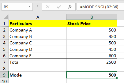
Just like Imply and Median, Mode will also be calculated within the Excel sheet as proven within the picture above. For instance, you possibly can put within the values of various firms within the Excel sheet and take out the Mode with the system =Mode.SNGL(B1: B5).
(B1: B5) – represents the values from cell B1 to B5.
Now, if we take the closing costs of Apple from Dec 26, 2018, to Dec 26, 2019, we’ll discover there isn’t a repeating worth, and therefore the mode of closing costs doesn’t exist as a result of inventory costs usually change daily and infrequently repeat precisely over an extended interval, particularly with the inclusion of decimal values.
Additionally, there may very well be a inventory that isn’t buying and selling in any respect; in such circumstances, the worth will stay fixed, making it straightforward to determine the mode. Moreover, for those who spherical inventory costs to the closest complete quantity, excluding decimal values, you’re more likely to discover a mode as sure rounded costs will seem extra continuously.
So whenever you attempt to calculate the Mode in Python with the next code:
It can throw the next error:
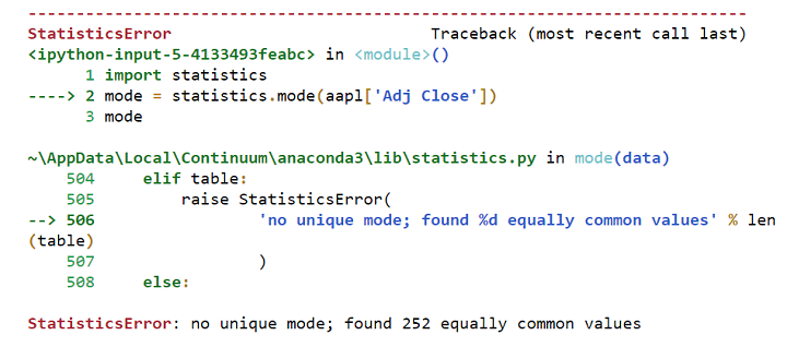
Therefore, the mode doesn’t make sense whereas observing closing value values.
Error in calculating mode
Therefore, the mode doesn’t make sense whereas observing closing value values. Coming to the importance of the mode, it’s most useful when it is advisable take out the repetitive inventory value from the earlier specific time interval. This time interval might be days, months and even years. Mainly, the mode of the information will provide help to perceive if the identical inventory value is anticipated to repeat sooner or later or not. Additionally, the mode is finest utilised whenever you wish to plot histograms and visualise the frequency distribution.
Wonderful! This brings you to the tip of the Measures of Central Tendency. Second, within the record of Descriptive Statistics is the Measure of Dispersion. Allow us to check out yet one more attention-grabbing idea.
Measure of Dispersion
You can find the that means of “Measure of Dispersion” proper in its title because it shows how scattered the information is across the central level. It merely tells the variation of every information worth from each other, which helps to offer a illustration of the distribution of the information. Additionally, it portrays the homogeneity and heterogeneity of the distribution of the observations.
Briefly, Measure of Dispersion reveals how a lot the complete information varies from their common worth.
The measure of dispersion might be divided into:
Now, allow us to perceive the idea of every class.
Vary
That is the most straightforward of all of the measures of dispersion and can also be straightforward to grasp. Vary merely implies the distinction between two excessive observations or numbers of the information set.
For instance, let X max and X min be two excessive observations or numbers. Right here, Vary would be the distinction between the 2 of them.Therefore,Vary = X max – X min
Additionally it is essential to notice that Quant analysts maintain a detailed comply with up on ranges. This occurs as a result of the ranges decide the entry in addition to exit factors of trades. Not solely the trades, however Vary additionally helps the merchants and traders in preserving a test on buying and selling intervals. This makes the traders and merchants bask in Vary-bound Buying and selling methods, which merely suggest following a specific trendline.
The trendlines are shaped by:
Excessive-priced shares (following an higher trendline) andLow-priced shares (following a decrease trendline)
On this the dealer should buy the safety on the decrease trendline and promote it at the next trendline to earn earnings. Therefore, in Python, this straightforward code will be capable to discover the wanted values for you:
The output is:
depend 250.000000
imply 170.633379
std 18.099152
min 123.998451
25% 159.071522
50% 174.227821
75% 184.849152
max 197.589523
Title: Adj Shut, dtype: float64
Allow us to check out how one other measure, Quartile Deviation features.
Quartile Deviation
That is the sort which divides a knowledge set into quarters. It consists of First Quartile as Q1, Second Quartile as Q2 and Third Quartile as Q3.
Right here,Q1 – is the quantity that comes between the smallest and the median of the information (1/4th) or the highest 25percentQ2 – is the median of the information orQ3 – is the quantity that comes between the median of knowledge and the biggest quantity (3/4th) or decrease 25percentn – is the entire variety of values
The system for Quartile deviation is: Q = ½ * (Q3 – Q1)
Since,Q1 is high 25%, the system for Q1 is – ¼ (n+1)Q3 can also be 25%, however the decrease one, so the system is – ¾ (n+1)Therefore, Quartile deviation = ½ * [(¾ (n+1) – ¼ (n+1)]
The foremost benefit, in addition to the drawback of utilizing this system, is that it makes use of half of the information to point out the dispersion from the imply or common. You should utilize the sort of measure of dispersion to review the dispersion of the observations that lie within the center. Any such measure of dispersion helps you perceive dispersion from the noticed worth and therefore, differentiates between the big values in numerous Quarters.
Within the monetary world, when it’s a must to examine a big information set (inventory costs) in numerous time intervals and wish to perceive the dispersed worth (costs) from an noticed one (average-median), Quartile deviation can be utilized.
The Python code right here is by assuming a collection of 10 random numbers:
The output is:
123.99845123291016
159.0715217590332
174.22782135009766
184.84915161132812
197.5895233154297
25.777629852294922
Nice, transferring forward Imply absolute deviation is yet one more measure which is defined forward.
Imply Absolute Deviation
Any such dispersion is the arithmetic imply of the deviations between the numbers in a given information set from their imply or median (common).
Therefore, the system of Imply Absolute Deviation is:
(D0 + D1 + D2 + D3 + D4 ….Dn)/ n
Right here,n = Complete variety of deviations within the information set andD0, D1, D2, and D3 are the deviations of every worth from the typical or median or imply within the information set andDn means the tip worth within the information set.
Explaining the Imply deviation, we’ll check out the picture under, which reveals a “computed imply” of a knowledge set and the distinction between every worth (within the dataset) from the imply worth. These variations or the deviations are proven as D0, D1, D2, and D3, …..D7.
For an occasion, if the imply values are as follows:

Then, the Imply right here might be calculated utilizing the imply system:3 + 6 + 6 + 7 + 8 + 11 + 15 + 16 / 8 = 9
Because the imply comes out to be 9, subsequent step is to seek out the deviation of every information worth from the Imply worth. So, allow us to compute the deviations, or allow us to subtract 9 from every worth to seek out D0, D1, D2, D3, D4, D5, D6, D7, and D8, which provides us the values as such:

As we at the moment are clear about all of the deviations, allow us to see the imply worth and all of the deviations within the type of a picture to get much more readability on the identical:
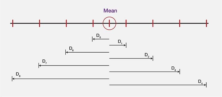
Therefore, from a big information set, the imply deviation represents the required values from noticed information worth precisely.
In python code, the computation of Imply deviation is as follows:
The output is 14.578809689453127
It is very important word that Imply deviation helps with a big dataset with numerous values which is very the case within the inventory market.
Going forward, variance is a associated idea and is additional defined.
Variance
Variance is a dispersion measure which suggests the typical of variations from the imply, in an analogous method as Imply Deviation does, however right here the deviations are squared.
So,$$Variance = [(DO)^2 + (D1)^2 + (D2)^2 + (D3)^2]/N$$
Right here,N = variety of values in information set andD0, D1, D2, D3 are the deviation of every worth within the information set from the imply.
Right here, taking the values from the instance above, we merely sq. every deviation after which divide the sum of deviated values by the entire quantity within the following method:$$(3)^2 + (6)^2 + (7)^2 + (8)^2 + (11)^2 + (15)^2 + (16)^2/8 = 99.5$$
In python code, it’s as follows:
The output is 326.26900384104425
Allow us to soar to a different measure referred to as Commonplace Deviation now.
Commonplace Deviation
In easy phrases, the usual deviation is a calculation of the unfold out of numbers in a knowledge set. The image (sigma)represents Commonplace deviation and the system is:$$σ = sqrt{Variance}$$
The system of ordinary deviation is:$$ σ = sqrt{frac{1}{N} sum_{i=1}^N (x_i – μ)^2$$
Right here, allow us to take the identical values as within the two examples above and calculate Variance. Therefore,$$σ = sqrt{99.5} = 9.97$$
Additional, in Python code, the usual deviation might be computed as follows:
The output is: 18.062917921560853
All of the kinds of measure of deviation carry out the required worth from the noticed one in a knowledge set in order to provide the good perception into totally different values of a variable, which might be value, time, and so forth. It is very important word that Imply absolute information, Variance and Commonplace Deviation, all assist in differentiating the values from common in a given massive information set.
Visualisation
Visualisation helps the analysts to resolve based mostly on organised information distribution. There are 4 such kinds of Visualisation method, that are:
Histogram

Age teams
Right here, within the picture above, you possibly can see the histogram with random information on x-axis (Age teams) and y-axis (Frequency). Because it seems at a big information in a summarised method, it’s primarily used for describing a single variable.
For an instance, x-axis represents Age teams from 0 to 100 and y-axis represents the Frequency of catching up with routine eye test up between totally different Age teams. The histogram illustration reveals that between the age group 40 and 50, frequency of individuals displaying up was highest.
Since histogram can be utilized for less than a single variable, allow us to transfer on and see how bar chart differs.
Bar chart
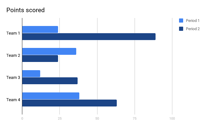
Within the picture above, you possibly can see the bar chart. Any such visualization lets you analyse the variable worth over a time period.
For an instance, the variety of gross sales in numerous years of various groups. You may see that the bar chart above reveals two years proven as Interval 1 and Interval 2.
In Interval 1 (first yr), Staff 2 and Staff 4 scored virtually the identical factors by way of variety of gross sales. And, Staff 1 was decently scoring however Staff 3 scored the least.In Interval 2 (second yr), Staff 1 outperformed all the opposite groups and scored the utmost, though, Staff 4 additionally scored decently nicely simply after Staff 1. Comparatively, Staff 3 scored decently nicely, whereas, Staff 2 scored the least.
Since this visible illustration can consider a couple of variable and totally different intervals in time, bar chart is sort of useful whereas representing a big information with numerous variables.
Allow us to now see forward how Pie chart is helpful in displaying values in a knowledge set.
Pie Chart
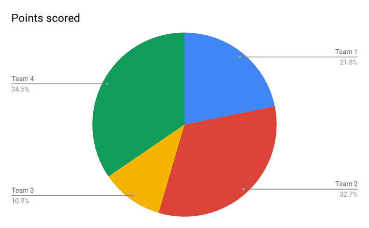
Above is the picture of a Pie chart, and this illustration lets you current the share of every variable from the entire information set. Every time you may have a knowledge set in proportion type and it is advisable current it in a method that it reveals totally different performances of various groups, that is the apt one.
For an instance, within the Pie chart above, it’s clearly seen that Staff 2 and Staff 4 have related efficiency with out even having to take a look at the precise numbers. Each the groups have outperformed the remainder. Additionally, it reveals that Staff 1 did higher than Staff 3. Since it’s so visually presentable, a Pie chart helps you in drawing an apt conclusion.
Shifting additional, the final within the collection is a Line chart.
Line chart
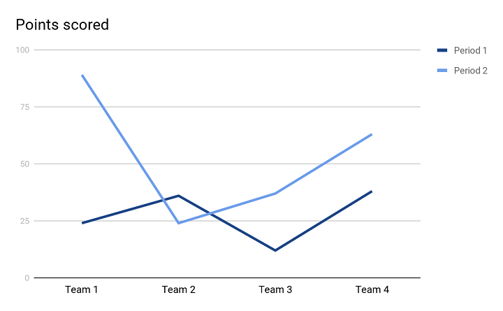
With this sort of illustration, the connection between two variables is clearer with the assistance of each y-axis and x-axis. This sort additionally lets you discover tendencies between the talked about variables.
Within the Line chart above, there are two development strains forming the visible illustration of 4 totally different groups in two Intervals (or two years). Each the development strains are serving to us be clear in regards to the efficiency of various groups in two years and it’s simpler to match the efficiency of two consecutive years. It clearly reveals that in Interval, 1 Staff 2 and Staff 4 carried out nicely. Whereas, in Interval 2, Staff 1 outperformed the remainder.
Okay, as we now have a greater understanding of Descriptive Statistics, we are able to transfer on to different mathematical ideas, their formulation in addition to functions in algorithmic buying and selling.
Likelihood Idea
Now allow us to return in time and recall the instance of discovering possibilities of a cube roll. That is one discovering that all of us have studied. Given the numbers on cube i.e. 1,2,3,4,5, and 6, the chance of rolling a 1 is 1 out of 6 or ⅙. Such a chance is named discrete through which there are a hard and fast variety of outcomes.
Now, equally, the chance of rolling a 2 is 1 out of 6, the chance of rolling a 3 can also be 1 out of 6, and so forth. A chance distribution is the record of all outcomes of a given occasion and it really works with a restricted set of outcomes in the way in which it’s talked about above. However, in case the outcomes are massive, features are for use.
If the chance is discrete, we name the perform a chance mass perform. Within the case of a cube roll, it will likely be:P(x) = 1/6 the place x = {1,2,3,4,5,6}
For discrete possibilities, there are specific circumstances that are so extensively studied, that their chance distribution has turn out to be standardised. Let’s take, for instance, Bernoulli’s distribution, which takes under consideration the chance of getting heads or tails after we toss a coin.
We write its chance perform as px (1 – p)(1 – x). Right here x is the end result, which may very well be written as heads = 0 and tails = 1.
Now, allow us to look into the Monte Carlo Simulation to grasp the way it approaches the chances sooner or later, taking a historic method.
Monte Carlo Simulation
It’s mentioned that the Monte Carlo methodology is a stochastic one (in which there’s sampling of random inputs) to unravel a statistical drawback. Properly merely talking, Monte Carlo simulation believes in acquiring a distribution of outcomes of any statistical drawback or information by sampling numerous inputs over and over. Additionally, it says that this manner we are able to outperform the market with none threat.
One instance of Monte Carlo simulation is rolling a cube a number of million occasions to get the consultant distribution of outcomes or doable outcomes. With so many doable outcomes, it will be practically unimaginable to go improper with the prediction of precise outcomes in future. Ideally, these checks are to be run effectively and rapidly which is what validates Monte Carlo simulation.
Though asset costs don’t work by rolling a cube, additionally they resemble a random stroll. Allow us to study Random Stroll now.
Random stroll
Random stroll means that the adjustments in inventory costs have the identical distribution and are impartial of one another. Therefore, based mostly on the previous development of a inventory value, future costs cannot be predicted. Additionally, it believes that it’s unimaginable to outperform the market with out bearing some quantity of threat. Coming again to the Monte Carlo simulation, it validates its personal principle by contemplating a variety of potentialities and on the belief that it helps cut back uncertainty.
Monte Carlo says that the issue is when just one roll of cube or a possible final result or a couple of extra are considered. Therefore, the answer is to match a number of future potentialities and customise the mannequin of belongings and portfolios accordingly.
After the Monte Carlo simulation, additionally it is vital to grasp Bayes’ theorem because it seems into the longer term possibilities based mostly on some relatable previous occurrences and therefore, has usability. In easy phrases, Bayes’ theorem shows the potential for the prevalence of an occasion based mostly on previous circumstances which may have led to a relatable occasion to happen.
For instance, say a specific age group between 50-55 had recorded most arthritis circumstances in months of December and January final yr and final to final yr additionally. Then it will likely be assumed that this yr as nicely in the identical months, the identical age group could also be identified with arthritis.
This may be utilized in chance principle, whereby, based mostly on previous occurrences with regard to inventory costs, future ones might be predicted.
There’s yet one more probably the most vital ideas of Arithmetic, often called Linear Algebra which now we’ll study.
Linear Algebra
Let’s study Linear Algebra in short.
What’s linear algebra?In easy phrases, linear algebra is the department of arithmetic that consists of linear equations, reminiscent of a1 x1 + ……. + an xn = b. A very powerful factor to notice right here is that Linear algebra is the arithmetic of knowledge, whereby, Matrices and Vectors are the core of knowledge.
What are matrices?A matrix or matrices is an accumulation of numbers organized in a specific variety of rows and columns. Numbers included in a matrix might be actual or complicated numbers or each.
For instance, M is a 3 by 3 matrix with the next numbers:
0 1 3
4 5 6
2 4 7
What are the vectors?In easy phrases, Vector is that idea of linear algebra that has each, a route and a magnitude.
For instance, ( mathbf{V} ) is:
[
mathbf{V} =
begin{bmatrix}
9
6
-5
end{bmatrix}
]
Now, If X =
$$[X_1]$$
$$[X_2]$$
$$[X_3]$$
Then, MX = V which is able to turn out to be ,
$$[0+X_2+3X_3] = [9]$$
$$[4X_1+5X_2+6X_3] = [6]; and$$
$$[2X_1+4X_2+7X_3] = [-5]$$
On this arrow, the purpose of the arrowhead reveals the route and the size of the identical is magnitude.
Above examples will need to have given you a good thought about linear algebra being all about linear combos. These combos make use of columns of numbers referred to as vectors and arrays of numbers often called matrices, which concludes in creating new columns in addition to arrays of numbers. There’s a identified involvement of linear algebra in making algorithms or in computations. Therefore, linear algebra has been optimized to fulfill the necessities of programming languages.
Additionally, for bettering effectivity, sure linear algebra implementations (BLAS and LAPACK) configure the algorithms in an automatic method. This helps the programmers to adapt to the precise nature of the pc system, like cache dimension, variety of cores and so forth.
In python code :
The output is:
rank of A: 3
Hint of A: 12
Determinant of A: 2.0000000000000004
Inverse of A: [[ 5.5 2.5 -4.5]
[-8. -3. 6. ]
[ 3. 1. -2. ]]
Matrix A raised to energy 3:
[[ 122 203 321]
[ 380 633 1002]
[ 358 596 943]]
Allow us to transfer forward to a different identified idea utilized in algorithmic buying and selling referred to as Linear Regression.
Linear Regression
Linear Regression is yet one more subject that helps in creating algorithms and is a mannequin which was initially developed in statistics. Linear Regression is an method for modelling the connection between a scalar dependent variable y and a number of explanatory variables (or impartial variables) denoted x.
However, regardless of being a statistical mannequin, it helps because the machine studying regression algorithm to foretell costs by displaying the connection between enter and output numerical variables.
How is Machine Studying useful in creating algorithms?
Machine studying implies an preliminary guide intervention for feeding the machine with applications for performing duties adopted by an computerized situation-based enchancment that the system itself works on. Briefly, Machine studying with its systematic method to foretell future occasions helps create algorithms for profitable automated buying and selling.
Calculating Linear Regression
The essential system of Linear Regression is: Y = mx+b
Beneath, you will note the representations of x & y clearly within the graph:
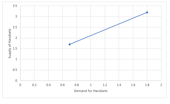
Within the graph above, the x-axis and y-axis each present variables (x and y). Since extra gross sales of handsets or demand (x-axis) of handsets are upsetting an increase in provide (y-axis) of the identical, a steep line is shaped. Therefore, to fulfill this rising demand, the availability or the variety of handsets additionally rises.
Merely,y = how a lot the development line goes up (Provide)x = how far the development line goes (Demand)b = intercept of y (the place the road crosses the y-axis)
In linear regression [²], the variety of enter values (x) are mixed to provide the expected output values (y) for that set of enter values. Each the enter values and output values are numeric.
Utilizing machine studying regression for buying and selling is defined briefly on this video under:
As we transfer forward, allow us to check out one other idea referred to as Calculus which can also be crucial for algorithmic buying and selling.
Calculus
Calculus is without doubt one of the principal ideas in algorithmic buying and selling and was truly termed infinitesimal calculus, which implies the examine of values which can be actually small to be even measured. On the whole, Calculus is a examine of steady change and therefore, essential for inventory markets as they maintain present process frequent adjustments.
Coming to the kinds of calculus, there are two broad phrases:
Differential Calculus: It calculates the instantaneous change in charges and the slopes of curves.Integral Calculus: This one calculates the portions summed up collectively.
In Calculus, we normally calculate the gap (d) in a specific time interval(t) as:
( d = at^2 )
the place,
( d ) is distance,
( a ) is acceleration, and
( t ) is time
Now, to simplify this calculation, allow us to suppose ( a = 5 ).
( d = 5t^2 )
Now, if time (( t )) is 1 second and distance coated is to be calculated on this time interval which is 1 second, then,
( d = 5(1)^2 = 5 , textual content{metres/second} )
Right here, it reveals that the gap coated in 1 second is 5 metres. However, if you wish to discover the pace at which 1 second was coated(present pace), then you will have a change in time, which might be t. Now, as it’s actually much less to be counted, t+t will denote o second.
Allow us to calculate the pace between t and t seconds as we all know from the earlier calculation that at 1 second, the gap coated was 5m/s. Now, with the identical system, we may even discover the gap coated at 0 seconds (t +t ):
So, ( d = 5t^2 )
( d = 5(t + t)^2 )
( d = 5(1 + t)^2 , textual content{m} )
Increasing ( (1 + t)^2 ), we’ll get ( 1 + 2t + t^2 )
( d = 5(1 + 2t + t^2) , textual content{m} )
( d = 5 + 10t + 5t^2 , textual content{m} )
Since, ( textual content{Velocity} = frac{textual content{distance}}{textual content{time}} )
( textual content{pace} = frac{5 + 10t + 5t^2 , textual content{m}}{t , textual content{s}} )
This brings us to the conclusion, ( 10 + 5t , textual content{m/s} )
Since t is taken into account to be a smaller worth than 1 second, and the pace is to be calculated at lower than a second (present pace), the worth of t might be near zero.Subsequently, the present pace = 10m/s
This examine of steady change might be appropriately used with linear algebra and in addition might be utilised in chance principle. In linear algebra, it may be used to seek out the linear approximation for a set of values. In chance principle, it might decide the potential for a steady random variable. Being part of regular distribution calculus can be utilized to seek out out regular distribution.
Superior! This brings us to the tip of all of the important mathematical ideas required for Quants/HFT/Algorithmic Buying and selling.
Conclusion
On this weblog, we explored the important function of arithmetic within the inventory market, beginning with primary inventory market maths and algorithmic buying and selling. We coated why arithmetic is significant for buying and selling algorithms, adopted by a historic perspective on its rise in finance.
Key mathematical ideas reminiscent of descriptive statistics, information visualisation, chance principle, and linear algebra had been mentioned. We additionally highlighted linear regression, its calculations, and the significance of machine studying in algorithm creation.
Lastly, we touched upon the relevance of calculus in monetary modelling. This information supplies a complete overview of how maths drives profitable inventory market buying and selling and algorithm growth.
In case you’re additionally desirous about creating lifelong abilities that may at all times help you in bettering your buying and selling methods. On this algorithmic buying and selling course, you’ll be educated in statistics & econometrics, programming, machine studying and quantitative buying and selling strategies, so you’re proficient in each talent essential to excel in quantitative & algorithmic buying and selling. Study extra in regards to the EPAT course now!
Creator: Chainika Thakar
Notice: The unique publish has been revamped on twenty first February 2024 for recentness, and accuracy.
Disclaimer: All information and data offered on this article are for informational functions solely. QuantInsti® makes no representations as to accuracy, completeness, currentness, suitability, or validity of any data on this article and won’t be accountable for any errors, omissions, or delays on this data or any losses, accidents, or damages arising from its show or use. All data is offered on an as-is foundation.
[ad_2]
Source link


, Boeing (NYSE:BA)")


